Reporting
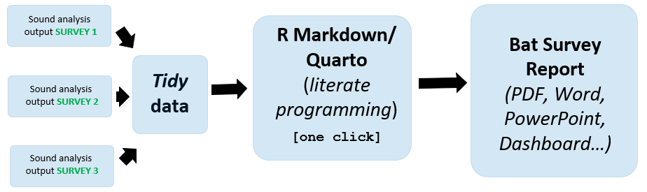
A full bat survey report produced, with one mouse click, from sound analysis data (i.e. after identifying the bat detector calls to species or genus with sound analysis) see Figure 1. One click reporting is achieved through literate programming (Knuth 1984); a procedure of mixing code and descriptive writing, in order to undertake and explain data analysis simultaneously in the same document. This is an efficient practice of workflow! A one click Word report see Section 2.1. A one click PowerPoint see Section 2.2.
1 Why Do This?
The advantages of this approach to bat data science are appreciable:
- Workflow
- Reduces (and can eliminate) any copy and paste activity
- Reports are easily created (one click) with new data or updated with revised data
- The time and effort producing reports can be reduced; by several orders of magnitude!
- Reproducible
- The report is reproducible by yourself (and others1); convenient when returning to a project after many months or years!
- The report is reproducible by yourself (and others1); convenient when returning to a project after many months or years!
- Open Source
- The Quarto or R Markdown file, the literate program document, is simple text that can be edited with any text editor; although it’s recommended to use friendly integrated development environments like RStudio2.
- The software3 which reads the literate program document and makes the report in: Word, PDF, PowerPoint or Dashboard are open source and free to use.
- The Quarto or R Markdown file, the literate program document, is simple text that can be edited with any text editor; although it’s recommended to use friendly integrated development environments like RStudio2.
What’s the disadvantage?
- Coding
- The literate program document requires coding skills to write (these web pages are designed to help with the coding).
- Coding skills in ecology are generally underdeveloped (although university education of ecology is increasingly taking a coding approach to data science); it should be noted little or no coding skills are required to render the report.
1.1 Evidence Led Reporting
Literate programming assists data science and reproducibility, promoting evidence led reporting and decision making. Reports are often produced for regulatory bodies, central government or local authorities, these organisations have mandatory strategies for the use of science, evidence and evaluation in there advice and actions, and the legality of their decisions(AUTOKEY?).
2 Bat Report from Tidy Data
2.1 Microsoft Word
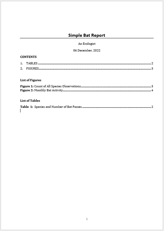
The complete R Markdown text (the .Rmd file) that produces a simple bat report from the statics tidy data4 is shown below; it can be copied to the clip board and rendered (knitted) into the Word report illustrated in Figure 2. The .Rmd file is also available here.
---
title: "Simple Bat Report"
output:
officedown::rdocx_document: default
date: "07 March, 2024"
author: "An Ecologist"
---
```{r include=FALSE}
library(knitr)
library(tidyverse)
library(iBats)
library(ggrepel)
library(broman)
library(flextable)
library(officer)
library(officedown)
library(treemapify)
library(ggthemes)
knitr::opts_chunk$set(echo = FALSE, warnings = FALSE, message = FALSE)
knitr::opts_chunk$set(fig.cap = TRUE)
# A vector used to give the species a specific colour in the graphic; the colours
# can be changed and other species added.
bat_colours_sci <- c(
"Barbastella barbastellus" = "#1f78b4",
"Myotis alcathoe" = "#a52a2a",
"Myotis bechsteinii" = "#7fff00",
"Myotis brandtii" = "#b2df8a",
"Myotis mystacinus" = "#6a3d9a",
"Myotis nattereri" = "#ff7f00",
"Myotis daubentonii" = "#a6cee3",
"Myotis spp." = "#bcee68",
"Plecotus auritus" = "#8b0000",
"Plecotus spp." = "#8b0000",
"Plecotus austriacus" = "#000000",
"Pipistrellus pipistrellus" = "#ffff99",
"Pipistrellus nathusii" = "#8a2be2",
"Pipistrellus pygmaeus" = "#b15928",
"Pipistrellus spp." = "#fdbf6f",
"Rhinolophus ferrumequinum" = "#e31a1c",
"Rhinolophus hipposideros" = "#33a02c",
"Nyctalus noctula" = "#cab2d6",
"Nyctalus leisleri" = "#fb9a99",
"Nyctalus spp." = "#eee8cd",
"Eptesicus serotinus" = "#008b8b"
)
```
__CONTENTS__
<!---BLOCK_TOC--->
__List of Figures__
<!---BLOCK_TOC{seq_id: 'fig'}--->
__List of Tables__
<!---BLOCK_TOC{seq_id: 'tab'}--->
```{r include=FALSE}
##### Load your TIDY bat data here:
# TidyBatData <- read_csv("YourTidyData.csv", col_names = TRUE)
# Tidy bat data - example data from the iBats package
TidyBatData <- statics
```
\newpage
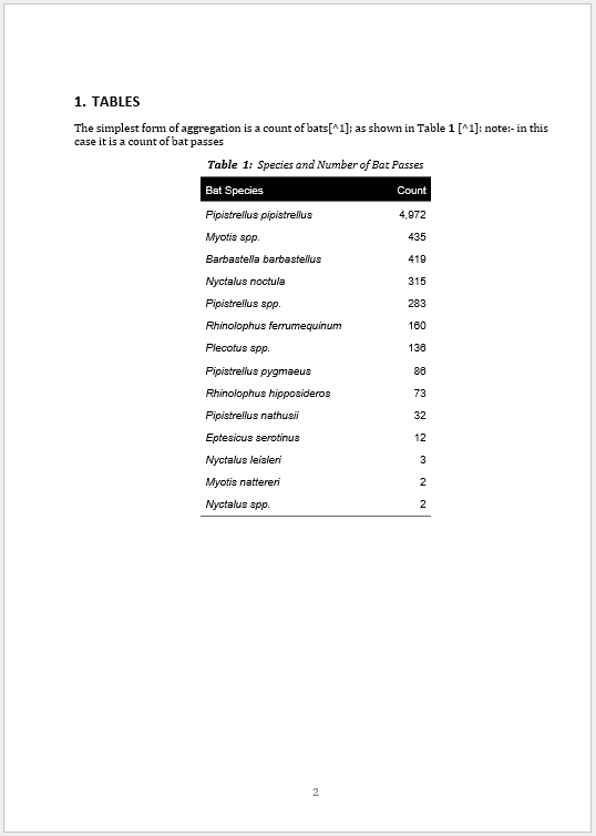
# TABLES
The simplest form of aggregation is a count of bats[^1]; as shown in Table \@ref(tab:table01)
[^1]: note:- in this case it is a count of bat passes
```{r tab.id="table01", tab.cap="Species and Number of Bat Passes"}
TidyBatData %>%
group_by(Species) %>%
count() %>%
#arrange descending
arrange(desc(n)) %>%
# rename n as count
rename(`Bat Species` = Species, Count = n) %>%
# so table is produced with individual species on one row
ungroup() %>%
flextable() %>%
width(j = 1, width = 2.5) %>%
italic(j = 1, italic = TRUE, part = "body") %>%
bg(bg = "black", part = "header") %>%
color(color = "white", part = "header")
```
\newpage
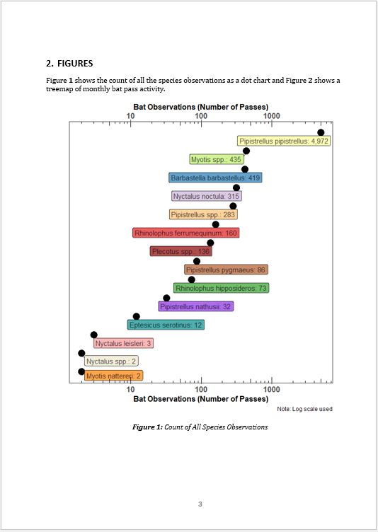
# FIGURES
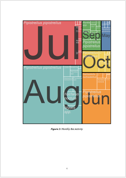
Figure \@ref(fig:graph01) shows the count of all the species observations as a dot chart and Figure \@ref(fig:graph02) shows a treemap of monthly bat pass activity.
```{r graph01, fig.cap="Count of All Species Observations", fig.height=7, fig.width=6}
g_data <- TidyBatData %>%
group_by(Species) %>%
count() %>%
mutate(total = add_commas(n),
label = stringr::str_c(Species, ": ", total))
graph_bat_colours <- iBats::bat_colours(g_data$Species, colour_vector = bat_colours_sci)
p <- ggplot(g_data, aes(y = reorder(Species, n), x = n, fill = Species)) +
geom_point(colour = "black", size = 5) +
geom_label_repel(data = g_data, aes(label = label),
nudge_y = -0.25,
nudge_x = ifelse(g_data$n < 100, 0.33, -0.33),
alpha = 0.7) +
scale_fill_manual(values = graph_bat_colours) +
scale_x_log10(sec.axis = dup_axis()) +
annotation_logticks(sides = "tb") +
labs(x = "Bat Observations (Number of Passes)",
caption = "Note: Log scale used") +
theme_bw() +
theme(legend.position = "none",
panel.grid.major = element_blank(),
panel.grid.minor = element_blank(),
axis.text.x = element_text(size=12, face="bold"),
axis.text.y = element_blank(),
axis.ticks.y = element_blank(),
strip.text = element_text(size=12, face="bold", colour = "white"),
axis.title.x = element_text(size=12, face="bold"),
axis.title.y = element_blank())
p
```
\newpage
```{r graph02, fig.cap="Monthly Bat Activity", fig.height=7, fig.width=6}
# Add data and time information to the iBats statics bat survey data set using the iBats::date_time_info
statics_plus <- iBats::date_time_info(statics)
graph_data <- statics_plus %>%
group_by(Species, Month) %>%
tally()
ggplot(graph_data, aes(area = n, fill = Month, label = Species, subgroup = Month)) +
scale_fill_tableau(palette = "Tableau 10") + #
geom_treemap(colour = "white", size = 2, alpha = 0.9) +
geom_treemap_subgroup_border(colour = "black", size = 5, alpha = 0.9) +
geom_treemap_subgroup_text(place = "centre", grow = T, alpha = 0.9, colour = "grey20", min.size = 0) +
geom_treemap_text(colour = "grey90", place = "topleft", fontface = "italic", reflow = T, min.size = 0, alpha = 0.9) +
theme_bw() +
theme(legend.position = "none") # No legend
```The three page Word report shown in Figure 2 is a rudimentary example; it could be expanded to include any of the tables and graphs shown on these web pages. The .Rmd file is rendered into a Microsoft Word document; this is a convenient file format easily allowing further editing by others in the survey team. The simple report in Figure 2 has a tables of contents and cross referencing it can also be rendered directly into the house/company style by specifying a reference_docx file5.
2.2 PowerPoint
The R Markdown text (the .Rmd file) that produces a PowerPoint presentation on the data files in the iBats package is shown below; it can be copied to the clip board and rendered (knitted) into the PowerPoint presentation illustrated in Figure 3. The .Rmd file is also available here.
---
date: "07 March 2024"
author: "Steve Markham"
title: "The iBats::_Data Files_"
output:
officedown::rpptx_document
---
```{r setup, include=FALSE}
knitr::opts_chunk$set(echo = FALSE, warnings = FALSE, message = FALSE)
library(officedown)
library(ggplot2)
library(rvg)
library(tidyverse)
library(flextable)
library(officer)
library(sf)
library(ggspatial)
library(rnaturalearth)
library(rnaturalearthdata)
library(iBats)
```
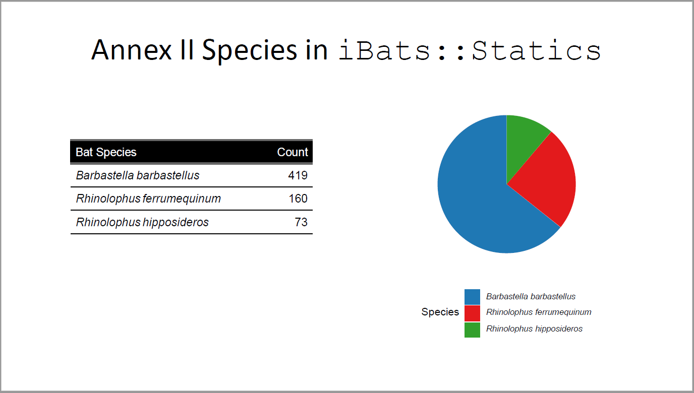
## Annex II Species in `iBats::Statics`
```{r layout='Two Content', ph=officer::ph_location_left()}
# Add data and time information to the statics data using the iBats::date_time_info
statics_plus <- iBats::date_time_info(statics)
AnnexII <- c("Barbastella barbastellus", "Rhinolophus ferrumequinum", "Rhinolophus hipposideros")
table_border <- fp_border(color = "black", width = 1) # from library(officer)
statics_plus %>%
filter(Species %in% AnnexII) %>%
group_by(Species) %>%
count() %>%
rename(`Bat Species` = Species, Count = n) %>%
flextable(col_keys = colnames(.)) %>%
italic(j = 1, italic = TRUE, part = "body") %>%
fontsize(part = "header", size = 12) %>%
fontsize(part = "body", size = 12) %>%
colformat_double(j = "Count", digits = 4, big.mark = ",") %>%
width(j = 1, width = 2.5) %>%
width(j = 2, width = 1) %>%
border_inner_h(part = "body", border = table_border) %>%
hline_bottom(part = "body", border = table_border) %>%
bg(bg = "black", part = "header") %>%
color(color = "white", part = "header")
```
```{r layout='Two Content', ph=officer::ph_location_right()}
graph_data <- statics_plus %>%
filter(Species %in% AnnexII) %>%
group_by(Species) %>%
count()
# colour values used by scale_fill_manual()
graph_bat_colours <- iBats::bat_colours_default(graph_data$Species)
mygg <- ggplot(graph_data, aes(x = "", y = n, fill = Species)) +
geom_bar(width = 1, stat = "identity") +
coord_polar(theta = "y") +
scale_fill_manual(values = graph_bat_colours) +
labs(
y = "Bat Pass Observations (Nr)",
fill = "Species"
) +
theme_bw() +
theme(
legend.position = "bottom",
legend.text = element_text(face = "italic"),
axis.text.x = element_blank(),
axis.text.y = element_blank(),
axis.ticks = element_blank(),
strip.text = element_blank(),
axis.title.x = element_blank(),
axis.title.y = element_blank(),
panel.grid.major = element_blank(),
panel.grid.minor = element_blank(),
panel.background = element_blank(),
panel.border = element_blank()
) +
guides(fill=guide_legend(ncol =1))
dml(ggobj = mygg)
```
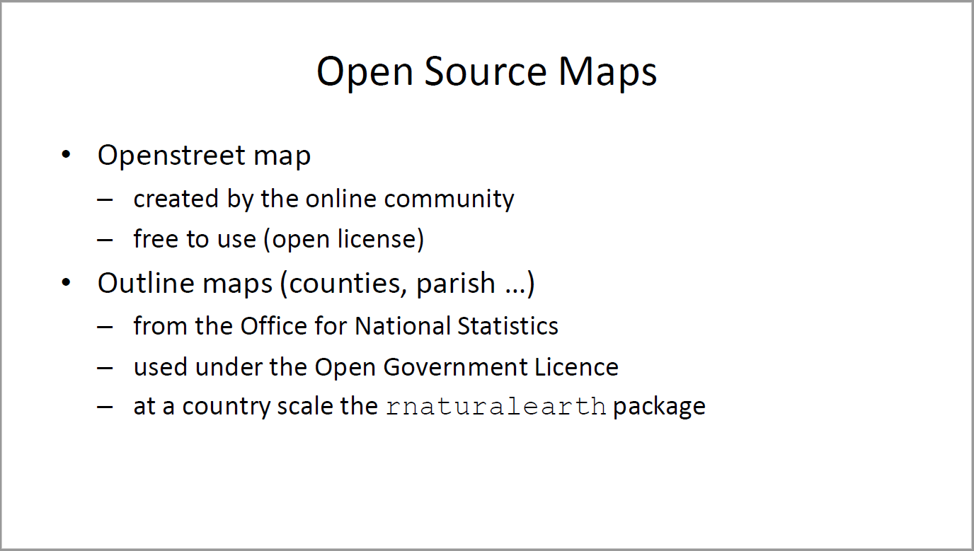
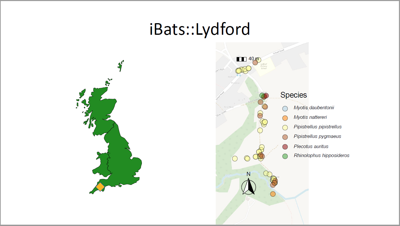
## Open Source Maps
- Openstreet map
- created by the online community
- free to use (open license)
- Outline maps (counties, parish ...)
- from the Office for National Statistics
- used under the Open Government Licence
- at a country scale the `rnaturalearth` package
## iBats::Lydford
```{r ph=officer::ph_location_left()}
#Outline maps countries
worldmap <- ne_countries(scale = 'medium', type = 'map_units',
returnclass = 'sf')
# GB only
GBcountires <- c("England", "Scotland", "Wales")
GB <- worldmap %>%
filter(name %in% GBcountires) %>%
select(geometry)
# Make location point for Mary Tavy Transect
MaryTavyLoc <- MaryTavy %>%
summarise(lat = median(`Latitude [WGS84]`),
lon = median(`Longitude [WGS84]`)) %>%
st_as_sf(coords = c("lon", "lat")) %>%
st_set_crs(4326) %>%
# Convert coord reference system to British National Grid
st_transform(crs = 27700)
p1 <- ggplot() +
geom_sf(data = GB,
linewidth = 0.25,
colour = "black",
fill = "#228b22") +
geom_sf(data = MaryTavyLoc,
shape = 23,
size = 6,
colour = "#00558e",
fill = "#fab824") +
theme_void()
dml(ggobj = p1)
```
```{r ph=officer::ph_location_left(), eval = FALSE}
# Make location point for Mary Tavy Transect
MaryTavyLoc <- MaryTavy %>%
summarise(lat = median(`Latitude [WGS84]`),
lon = median(`Longitude [WGS84]`)) %>%
st_as_sf(coords = c("lon", "lat")) %>%
st_set_crs(4326) %>%
# Convert coord reference system to British National Grid
st_transform(crs = 27700)
# Load outline map
GB <- sf::st_read("maps/GeneralGB/CTYUA_Dec_2017_GCB_GB.shp", quiet = TRUE) %>%
filter(ctyua17nm == "Devon")
# Plot map and Location
p2 <- ggplot() +
geom_sf(data = GB,
linewidth = 0.25,
colour = "#228b22",
fill = "#98FB98") +
geom_sf(data = MaryTavyLoc,
shape = 23,
size = 3,
colour = "#00558e",
fill = "#fab824") +
labs(title = "Devon") +
theme_void() +
theme(title = element_text(colour = "#228b22", size = 14, face = "bold"))
dml(ggobj = p2)
```
```{r ph=officer::ph_location_right()}
spatial_data <- Lydford%>%
select(Species, longitude = Longitude, latitude = Latitude)
# default colour values used by scale_fill_manual() - scientific names - UK bats only
graph_bat_colours <- iBats::bat_colours_default(spatial_data$Species)
spatial_data <- st_as_sf(spatial_data, coords = c("longitude", "latitude"),
crs = 4326)
p1 <- ggplot() +
annotation_map_tile(type = "osm", zoomin = -1, alpha = 0.5) +
geom_sf(data = spatial_data, aes(fill = Species), shape = 21, alpha = 0.5, size = 4) +
annotation_scale(location = "tl") +
annotation_north_arrow(location = "bl",
which_north = "true",
style = north_arrow_fancy_orienteering()) +
# fixed_plot_aspect(ratio = 1) +
coord_sf() +
scale_fill_manual(values = graph_bat_colours) +
scale_size_area(max_size = 12) +
theme_void() +
theme(legend.position = "right",
axis.title.y = element_blank(),
axis.title.x = element_blank(),
axis.text.x = element_blank(),
axis.text.y = element_blank(),
axis.ticks = element_blank(),
title = element_text(colour = "black", size = 14),
legend.text = element_text(face = "italic"))
dml(ggobj = p1)
```
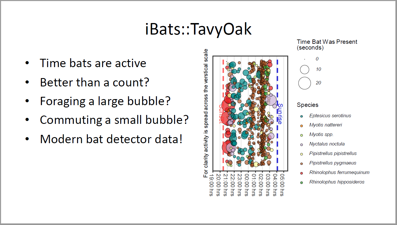
## iBats::TavyOak
- Time bats are active
- Better than a count?
- Foraging a large bubble?
- Commuting a small bubble?
- Modern bat detector data!
```{r ph=officer::ph_location_right()}
bat_colours_sci <- c(
"Barbastella barbastellus" = "#1f78b4",
"Myotis alcathoe" = "#a52a2a",
"Myotis bechsteinii" = "#7fff00",
"Myotis brandtii" = "#b2df8a",
"Myotis mystacinus" = "#6a3d9a",
"Myotis nattereri" = "#ff7f00",
"Myotis daubentonii" = "#a6cee3",
"Myotis spp." = "#bcee68",
"Plecotus auritus" = "#8b0000",
"Plecotus spp." = "#8b0000",
"Plecotus austriacus" = "#000000",
"Pipistrellus pipistrellus" = "#ffff99",
"Pipistrellus nathusii" = "#8a2be2",
"Pipistrellus pygmaeus" = "#b15928",
"Pipistrellus spp." = "#fdbf6f",
"Rhinolophus ferrumequinum" = "#e31a1c",
"Rhinolophus hipposideros" = "#33a02c",
"Nyctalus noctula" = "#cab2d6",
"Nyctalus leisleri" = "#fb9a99",
"Nyctalus spp." = "#eee8cd",
"Eptesicus serotinus" = "#008b8b"
)
# graph anotation
graph_sunrise <- TavyOak$sunrise[1]
graph_sunset <- TavyOak$sunset[1]
# graph time limits x-axis
graph_limit1 <- TavyOak$sunset[1] - lubridate::hours(1)
graph_limit2 <- TavyOak$sunrise[1] + lubridate::hours(1)
# colour values used by scale_fill_manual()
graph_bat_colours <- iBats::bat_colours(TavyOak$Species, colour_vector = bat_colours_sci)
mygg <- ggplot(TavyOak, aes(y = 1, x = DateTime, fill = Species, size = bat_time)) +
geom_jitter(shape = 21, alpha = 0.7) +
geom_vline(
xintercept = graph_sunset,
colour = "brown1",
linetype = "dashed",
linewidth = 1,
alpha = 0.8
) +
geom_vline(
xintercept = graph_sunrise,
colour = "mediumblue",
linetype = "dashed",
linewidth = 1,
alpha = 0.8
) +
annotate("text",
x = graph_sunset - lubridate::minutes(20),
y = 1,
label = "Sunset",
color = "brown1",
angle = 270
) +
annotate("text",
x = graph_sunrise + lubridate::minutes(20),
y = 1,
label = "Sunrise",
color = "mediumblue",
angle = 270
) +
scale_fill_manual(values = graph_bat_colours) +
scale_size_area(max_size = 12) +
scale_x_datetime(
date_labels = "%H:%M hrs",
date_breaks = "1 hour",
limits = c(graph_limit1, graph_limit2)
) +
labs(
fill = "Species",
size = "Time Bat Was Present\n(seconds)",
y = "For clarity activity is spread across the verstical scale"
) +
theme_bw() +
theme(
legend.position = "right",
panel.grid.major.x = element_line(),
panel.grid.major.y = element_blank(),
panel.grid.minor = element_blank(),
axis.text.x = element_text(size = 10, angle = 270),
axis.text.y = element_blank(),
axis.ticks.y = element_blank(),
strip.text = element_text(size = 12, face = "bold", colour = "white"),
legend.text = element_text(face = "italic"),
axis.title.x = element_blank(),
axis.title.y = element_text(size = 10)
)
dml(ggobj = mygg)
```
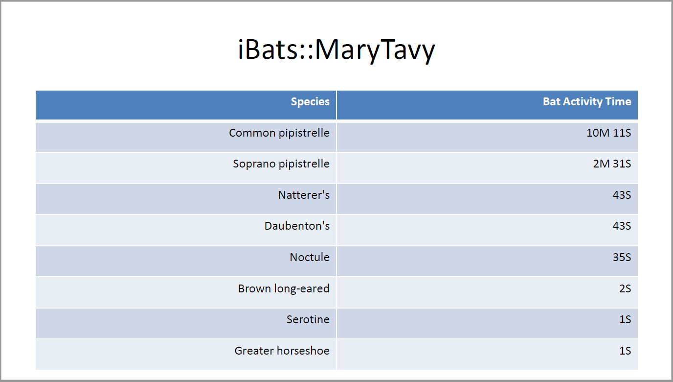
## iBats::MaryTavy
```{r layout='Title and Content', ph=officer::ph_location_type(type="body")}
###############################################################################
# MaryTavy is data directly exported from BatExplorer and requires tidying!####
###############################################################################
#### Combine the two Species columns into one ##################################
# Select Species column and remove (Species2nd & Species3rd)
data1 <- MaryTavy %>%
select(-`Species 2nd Text`) %>%
rename(Species = `Species Text`)
# Select Species2nd column and remove (Species & Species3rd)
data2 <- MaryTavy %>%
select(-`Species Text`) %>%
filter(`Species 2nd Text` != "-") %>% # Remove blank rows
rename(Species = `Species 2nd Text`) # Rename column
# Add the datasets together into one
MaryTavyTidying <- dplyr::bind_rows(data1, data2)
################################################################################
#### Calculate bat activity time and prepare to make spatial data #############
tidy_data <- MaryTavyTidying %>%
mutate(calls = `Calls [#]`,
duration = `Mean Call Lenght [ms]`,
span = `Mean Call Distance [ms]`,
# Calculate BatActivityTime in seconds
bat_time = calls * (duration + span) / 1000) %>%
select(Species, bat_time)
#Make species have common names
tidy_data$Species <- bat_common_default(tidy_data$Species)
# Aggregate data into Species and count
tidy_data %>%
group_by(Species) %>%
summarise(bat_time = sum(bat_time)) %>%
arrange(desc(bat_time)) %>%
mutate(bat_time = round(bat_time, digits = 0),
bat_time = lubridate::seconds_to_period(bat_time)) %>%
rename(`Bat Activity Time` = bat_time)
```
References
Footnotes
the exact results can be reproduced if given access to the original data and Quarto® document containing the literate programming text of code and descriptive writing.↩︎
RStudio is now known as Posit https://posit.co/; and now embraces R and Python.↩︎
e.g. R https://www.r-project.org/, Python https://www.python.org/, R Markdown https://rmarkdown.rstudio.com/, Quarto® https://quarto.org/, RStudio https://posit.co/, Jupyter https://jupyter.org/.↩︎
From the iBats package.↩︎
More information on the production of Word documents and PowerPoint presentations from R and R Markdown is available from the work of David Gohel see https://ardata-fr.github.io/officeverse/index.html.↩︎