Tidy Data is a consistent way to organise your data (Wickham 2014)(Tierney and Cook 2023). Getting your data into this format requires some initial work, but that effort pays off in the long term. Once you have tidy data you will spend less time wrangling data from one representation to another, allowing you to spend more time on the analytic questions at hand. Unfortunately, there is a rule of thumb; 80% of time doing data science is spent wrangling data; particularly the effort required in sorting and rearranging the data into the tidy and therefore usable format; illustrated below are ways to make this task less demanding.
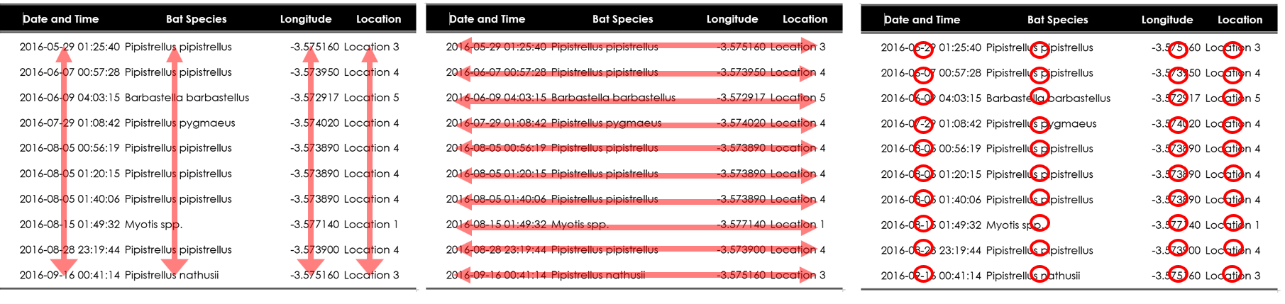
There are three interrelated rules which make a data set tidy see Figure 1:
Each variable must have its own column.
Each observation must have its own row.
Each value must have its own cell.
Figure 1: Rules for Tidy Data
1 Minimal Data Requirement
To undertake meaningful data analysis, it is recommended that data collected from bat activity surveys is wrangled into tidy data that has the following five variables (columns) as a minimum and illustrated in Table 1:
Description
DateTime
Species
Latitude
Longitude
The rationale for these variables is as follows:
Description a column to help identify the observation for example a location, surveyor or survey number.
Always Use a Description
Although a description column is not absolutely necessary for a minimal data set. Description column(s) portraying the location, survey number or surveyor gives both the data and the analysis context.
DateTime: the date and time of the bat observation to BS ISO 8601:2004 i.e. yyyymmdd hh:mm:ss. The use of BS ISO 8601:2004 prevents confusion over the date format 1 . Reference bat activity to the local time and specifying an iana2 time zone allows for daylight saving times to considered; the iana code for the UK is Europe/London.
Species: bat species names should follow the “binomial nomenclature” from the International Code of Zoological Nomenclature (ICZN)3 - e.g. Barbastella barbastellus, Eptesicus serotinus, etc… A column of local common names can always be added to the tidy data, i.e. in a separate column see Meta Data. A compiled online database Bats of the World provides taxonomic and geographic information on all Chiroptera 4. As of 10th Mar 2023, 1462 species are recognized. Sound analysis may not be able to distinguish calls to species level; in practice some calls may only be identified to genus or as acoustically similar, Table 13 suggests a naming convention.
Longitude and Latitude: World Geodetic System 19845 (WGS84); as used by Google earth. A digital, numeric, format should be used. Any other spatial reference system can be used, as these can be stored as an extra column in the tidy data; an example of British National Grid co-ordinates (Easting/Northing) is provided in Meta Data. The prerequisite is that the reference system can be converted to WGS84; which is the case for most national or state co-ordinate systems. Using a global co-ordinate system such as WSG84 gives access to the many open-source application programming interfaces (API) available that assist with data analysis (e.g. assessing sunset and sunrise times or the adjustment to daylight saving).
Code
library(tidyverse)library(iBats)library(gt)statics %>%# statics is a tidy data set from the iBats packageselect(Description, DateTime, Species, Latitude, Longitude) %>%sample_n(10) %>%arrange(DateTime) %>%# Table made with gt()gt() %>%tab_style(style =list(cell_fill(color ="black"),cell_text(color ="white", weight ="bold") ),locations =cells_column_labels(columns =c(everything()) ) ) %>%# Make bat scientific name italictab_style(style =list(cell_text(style ="italic") ),locations =cells_body(columns =c(Species) ) ) %>%# reduce cell spacetab_options(data_row.padding =px(2)) %>%cols_align(align ="left",columns = DateTime )
two of more columns with species of same date and time (Table 6);
code names for species rather than the binomial nomenclature (Table 3); and,
Longitude and Latitude columns with missing values (Table 9)
While the bat survey results shown in Table 1 is an example of a tidy data set; the data shown in Table 2, Table 4, Table 6, Table 3 and, Table 9 are untidy and would need to be made tidy to undertake analysis.
Data preparation is not just a first step but must be repeated many times over during analysis; as new problems come to light, or new data is collected. Making bat data into a tidy format, involves cleaning data: parsing dates and numbers, identifying missing values, correcting character encoding, matching similar but not identical values (such as those created by typos); it is an essential step, takes time to do and makes subsequent steps in the analysis much easier.
Too many species in a cell, as in Table 2, can be made tidy by expanding the data so each species observed is in it’s own row, using the function tidyr::separate_rows(Species); as shown below in Table 3. Note that this data has untidy bat names; these are corrected in Section 2.4. The untidy1 data is example untidy data available from the iBats package.
Code
### Libraries Usedlibrary(tidyverse) # Data Science packages - see https://www.tidyverse.org/library(gt) # Makes table# Install devtools if not installed# devtools is used to install the iBats package from GitHubif (!require(devtools)) {install.packages("devtools")}# If iBats is not installed load from Githubif (!require(iBats)) { devtools::install_github("Nattereri/iBats")}library(iBats)untidy1 %>% tidyr::separate_rows(Species) %>%# Table made with gt()gt() %>%tab_style(style =list(cell_fill(color ="black"),cell_text(color ="white", weight ="bold") ),locations =cells_column_labels(columns =c(everything()) ) ) %>%# reduce cell spacetab_options(data_row.padding =px(2)) %>%cols_align(align ="left",columns = DateTime )
Untidy Bat Data a Column Giving the Number of Bat Passes
DateTime
Species
Number
2019-10-05 20:35:15
Pipistrellus pipistrellus
1
2019-10-05 20:38:30
Pipistrellus pygmaeus
1
2019-10-05 20:49:40
Nyctalus noctula
2
2019-10-05 21:05:15
Pipistrellus pipistrellus
1
2019-10-05 21:15:30
Pipistrellus pygmaeus
3
2019-10-05 21:25:45
Pipistrellus pipistrellus
1
A count of species, as in Table 4, can be made tidy by un-counting the data so each species observed is in it’s own row, using the function tidyr::uncount(Number); as shown below in Table 5. The untidy2 data is example untidy data available from the iBats package.
Code
### Libraries Usedlibrary(tidyverse) # Data Science packages - see https://www.tidyverse.org/library(gt) # Makes table# Install devtools if not installed# devtools is used to install the iBats package from GitHubif (!require(devtools)) {install.packages("devtools")}# If iBats is not installed load from Githubif (!require(iBats)) { devtools::install_github("Nattereri/iBats")}library(iBats)untidy2 %>% tidyr::uncount(Number) %>%# Table made with gt()gt() %>%tab_style(style =list(cell_fill(color ="black"),cell_text(color ="white", weight ="bold") ),locations =cells_column_labels(columns =c(everything()) ) ) %>%# reduce cell spacetab_options(data_row.padding =px(2)) %>%cols_align(align ="left",columns = DateTime )
Several columns of species, as in Table 6, can be made tidy by making separate data.frames and binding them together so each species observed is in it’s own row; as shown below in Table 7. The untidy3 data is example untidy data available from the iBats package.
Code
### Libraries Usedlibrary(tidyverse) # Data Science packages - see https://www.tidyverse.org/# Install devtools if not installed# devtools is used to install the iBats package from GitHubif (!require(devtools)) {install.packages("devtools")}# If iBats is not installed load from Githubif (!require(iBats)) { devtools::install_github("Nattereri/iBats")}library(iBats)# Select Species column and remove (Species2nd & Species3rd)data1 <- untidy3 %>%select(-Species2nd, -Species3rd)# Select Species2nd column and remove (Species & Species3rd)data2 <- untidy3 %>%select(-Species, -Species3rd) %>%filter(Species2nd !="") %>%# Remove blank rowsrename(Species = Species2nd) # Rename column# Select Species3rd column and remove (Species & Species2nd)data3 <- untidy3 %>%select(-Species, -Species2nd) %>%filter(Species3rd !="") %>%# Remove blank rowsrename(Species = Species3rd) # Rename column# Add the datasets together into onedplyr::bind_rows(data1, data2, data3) %>%# Table made with gt()gt() %>%tab_style(style =list(cell_fill(color ="black"),cell_text(color ="white", weight ="bold") ),locations =cells_column_labels(columns =c(everything()) ) ) %>%# reduce cell spacetab_options(data_row.padding =px(2)) %>%cols_align(align ="left",columns = DateTime )
Table 7:
Tidied Bat Data with Two or More Columns put into One
DateTime
Species
2019-10-04 20:35:15
Common pipistrelle
2019-10-04 20:38:30
Soprano pipistrelle
2019-10-04 21:05:15
Common pipistrelle
2019-10-04 21:15:30
Soprano pipistrelle
2019-10-04 21:25:45
Common pipistrelle
2019-10-04 20:38:30
Noctule
2019-10-04 21:15:30
Common pipistrelle
2019-10-04 21:25:45
Common pipistrelle
2019-10-04 21:15:30
Noctule
2.4 Convert Bat Names to Scientific
Table 3 is still untidy because the bat species are represented as codes and not in a binomial nomenclature(scientific name). The iBats::make_scientific() function can take a named vector of codes and the scientific name; such as the BatScientific vector below. The case of the bat name codes are ignored; they are all converted to lower case.
Code
BatScientific <-c("nyclei"="Nyctalus leisleri","nycnoc"="Nyctalus noctula","pippip"="Pipistrellus pipistrellus","pipnat"="Pipistrellus nathusii","pippyg"="Pipistrellus pygmaeus","45 pip"="Pipistrellus pipistrellus","55 pip"="Pipistrellus pygmaeus","bleb"="Plecotus auritus",# If already a scientific name keep it"myotis daubentonii"="Myotis daubentonii")
The BatScientific vector is then used to covert the survey vector of bat names (the Species column in Table 3) so they are all scientific; using the iBats::make_scientific() function. The BatScientific can be expanded to cover many names and codes, if there are duplicate names or codes a conversion will not take place for that name or code. The tidied data with scientific species names is shown in Table 8
Code
### Libraries Used library(tidyverse) # Data Science packages - see https://www.tidyverse.org/# Install devtools if not installed # devtools is used to install the iBats package from GitHubif(!require(devtools)){install.packages("devtools")}# If iBats is not installed load from Githubif(!require(iBats)){ devtools::install_github("Nattereri/iBats")}library(iBats)# Remove too many species in a celltidied1 <- untidy1 %>% tidyr::separate_rows(Species)tidied1$Species <- iBats::make_scientific(BatScientific, tidied1$Species)
Code
library(gt)# Table made with gt()tidied1 %>%gt() %>%tab_style(style =list(cell_fill(color ="black"),cell_text(color ="white", weight ="bold") ),locations =cells_column_labels(columns =c(everything()) ) ) %>%# Make bat scientific name italictab_style(style =list(cell_text(style ="italic") ),locations =cells_body(columns =c(Species) )) %>%# reduce cell spacetab_options(data_row.padding =px(2)) %>%cols_align(align ="left",columns = DateTime )
Table 8:
Tidied Data with Scientific Names
DateTime
Species
2019-10-03 20:55:30
Pipistrellus pygmaeus
2019-10-03 20:58:30
Pipistrellus pygmaeus
2019-10-03 20:58:30
Nyctalus leisleri
2019-10-03 21:15:30
Pipistrellus pygmaeus
2019-10-03 21:25:30
Pipistrellus pipistrellus
2019-10-03 21:25:30
Pipistrellus pygmaeus
2019-10-03 21:25:30
Nyctalus leisleri
2019-10-03 21:35:30
Pipistrellus pipistrellus
2.5 Missing Latitude and Longitude Values
The BatExplorer data in the iBats package (see Table 9), was recorded on an evening transect bat detector survey. The data has missing longitude and latitude values, shown as NA and is not uncommon when the Global Positioning System (GPS) is trying to calculate its position beneath trees or in a steep valley.
Code
### Libraries Used library(tidyverse) # Data Science packages - see https://www.tidyverse.org/library(iBats)library(gt)# BatExplorer csv file is from the iBats packageBatExplorer %>%head(n=15L) %>%select(DateTime = Timestamp, Species =`Species Text`, Latitude =`Latitude [WGS84]`,Longitude =`Longitude [WGS84]`) %>%# Table made with gt()gt() %>%tab_style(style =list(cell_fill(color ="black"),cell_text(color ="white", weight ="bold") ),locations =cells_column_labels(columns =c(everything()) ) ) %>%# Make bat scientific name italictab_style(style =list(cell_text(style ="italic") ),locations =cells_body(columns =c(Species) )) %>%# reduce cell spacetab_options(data_row.padding =px(2)) %>%cols_align(align ="left",columns = DateTime )
Table 9:
Missing Longitude and Latitude Values (NA)
DateTime
Species
Latitude
Longitude
06/05/2018 21:05:24
Pipistrellus pygmaeus
NA
NA
06/05/2018 21:06:51
Nyctalus noctula
NA
NA
06/05/2018 21:09:23
Nyctalus noctula
NA
NA
06/05/2018 21:13:20
Nyctalus noctula
NA
NA
06/05/2018 21:19:16
Pipistrellus pygmaeus
50.51771
-4.162705
06/05/2018 21:20:33
Pipistrellus pygmaeus
50.51704
-4.162595
06/05/2018 21:20:40
Pipistrellus pygmaeus
50.51706
-4.162693
06/05/2018 21:31:51
Pipistrellus pygmaeus
50.54168
-4.188790
06/05/2018 21:32:35
Pipistrellus pygmaeus
NA
NA
06/05/2018 21:34:00
Nyctalus noctula
NA
NA
06/05/2018 21:34:02
Nyctalus noctula
NA
NA
06/05/2018 21:34:04
Nyctalus noctula
NA
NA
06/05/2018 21:34:14
Nyctalus noctula
50.51703
-4.162153
06/05/2018 21:34:27
Pipistrellus pipistrellus
50.51703
-4.162153
06/05/2018 21:35:27
Rhinolophus hipposideros
50.49506
-4.137962
The longitude and latitude gives a position of the bat observation and is also used to determine sunset and sunrise; and if the values are not completed then these observations would be excluded from the analysis. A simple estimate of the missing latitude and longitude can be made by arranging the data in date/time order and using the function:
This fills the missing values from the nearest complete values; first down and then up. The filled data is shown in Table 10.
Warning
Latitude and longitude is required in every row for the sun times can be calculated.
Code
### Libraries Usedlibrary(tidyverse) # Data Science packages - see https://www.tidyverse.org/# Install devtools if not installed# devtools is used to install the iBats package from GitHubif (!require(devtools)) {install.packages("devtools")}# If iBats is not installed load from Githubif (!require(iBats)) { devtools::install_github("Nattereri/iBats")}library(iBats)# BatExplorer csv file is from the iBats packageBatExplorer %>%head(n = 15L) %>%select(DateTime = Timestamp,Species =`Species Text`,Latitude =`Latitude [WGS84]`,Longitude =`Longitude [WGS84]` ) %>%arrange(DateTime) %>% tidyr::fill(c(Latitude, Longitude), .direction ="downup")
Code
# BatExplorer csv file is from the iBats packageBatExplorer %>%head(n=15L) %>%select(DateTime = Timestamp, Species =`Species Text`, Latitude =`Latitude [WGS84]`,Longitude =`Longitude [WGS84]`) %>%fill(Latitude, .direction ="downup") %>%fill(Longitude, .direction ="downup") %>%gt() %>%tab_style(style =list(cell_fill(color ="black"),cell_text(color ="white", weight ="bold") ),locations =cells_column_labels(columns =c(everything()) ) ) %>%# Make bat scientific name italictab_style(style =list(cell_text(style ="italic") ),locations =cells_body(columns =c(Species) )) %>%# reduce cell spacetab_options(data_row.padding =px(2)) %>%cols_align(align ="left",columns = DateTime )
Table 10:
Filled Longitude and Latitude Values
DateTime
Species
Latitude
Longitude
06/05/2018 21:05:24
Pipistrellus pygmaeus
50.51771
-4.162705
06/05/2018 21:06:51
Nyctalus noctula
50.51771
-4.162705
06/05/2018 21:09:23
Nyctalus noctula
50.51771
-4.162705
06/05/2018 21:13:20
Nyctalus noctula
50.51771
-4.162705
06/05/2018 21:19:16
Pipistrellus pygmaeus
50.51771
-4.162705
06/05/2018 21:20:33
Pipistrellus pygmaeus
50.51704
-4.162595
06/05/2018 21:20:40
Pipistrellus pygmaeus
50.51706
-4.162693
06/05/2018 21:31:51
Pipistrellus pygmaeus
50.54168
-4.188790
06/05/2018 21:32:35
Pipistrellus pygmaeus
50.54168
-4.188790
06/05/2018 21:34:00
Nyctalus noctula
50.54168
-4.188790
06/05/2018 21:34:02
Nyctalus noctula
50.54168
-4.188790
06/05/2018 21:34:04
Nyctalus noctula
50.54168
-4.188790
06/05/2018 21:34:14
Nyctalus noctula
50.51703
-4.162153
06/05/2018 21:34:27
Pipistrellus pipistrellus
50.51703
-4.162153
06/05/2018 21:35:27
Rhinolophus hipposideros
50.49506
-4.137962
3 Output from Sound Analysis Software
The output from proprietary sound analysis software (e.g. BatExplorer, Kaleidoscope …) vary in format and content with significant differences in:
column headings
naming of bats
format of date and time
This makes the output from the different software cumbersome to join together and undertake analysis. This barrier to data analysis can be overcome by manipulating the output, so it contains at least the minimal data columns shown in Table 1.
When combining data obtained in the field from varying bat detectors and then processed with a range of sound analysis software it’s important record this meta information in tidy columns for every record.
It is recommended the data exported from the sound analysis software is a comma separated value *.csv file.
The Original Information is Retained.
During manipulation all the original data in the software’s exported *.csv is retained. For example any columns holding the meta information, e.g. the recording ID.
3.1 Elekon AG BatExplorer
The exported .csv output from BatExplorer has the following columns requiring manipulation to create minimal data (an outline of the the manipulation is described in the brackets):
Timestamp - (rename or copy column to DateTime and check date is BS ISO 8601:2004 yyyymmdd hh:mm:ss format)
Species Text - (rename or copy column to Species, the text is normally exported as a scientific name)
Latitude [WGS84] - (rename or copy column to Latitude)
Longitude [WGS84] - (rename or copy column to Longitude)
section under-construction
3.2 BTO Acoustic Pipeline
The exported .csv output from the BTO Acoustic Pipeline has the following columns requiring manipulation to create minimal data (an outline of the the manipulation is described in the brackets):
ACTUAL DATE, TIME - (combine ACTUAL DATE and TIME into DateTime convert date to BS ISO 8601:2004 yyyymmdd hh:mm:ss format)
SCIENTIFIC NAME - (rename or copy column to Species)
LATITUDE - (rename or copy column to Latitude)
LONGITUDE - (rename or copy column to Longitude)
The iBats package has the Static_G dataset an exported .csv file from the BTO Acoustic Pipeline. The code below shows how to make minimal data from Static_G; the first ten lines are produced in Table 11.
Code
# minimal data minimal_Static_G <- Static_G %>%mutate(DateTime =glue("{`ACTUAL DATE`} {TIME}"), # combine date and timeDateTime = lubridate::dmy_hms(DateTime), # make an ISO date (check format is dmy)Species =`SCIENTIFIC NAME`, # Species nameLatitude =`LATITUDE`,Longitude =`LONGITUDE`,Description ="Static G") %>%# add a description# Note the everything() function retains all the original informationselect(Description, DateTime, Species, Latitude, Longitude, everything()) #
The exported .csv output from the Kaleidoscope has the following columns requiring manipulation to create minimal data (an outline of the the manipulation is described in the brackets):
DATE, TIME - (combine DATE and TIME into DateTime convert date to BS ISO 8601:2004 yyyymmdd hh:mm:ss format)
AUTO-ID or MANUAL ID - (rename or copy column to Species; multiple species in a cell, separate into separate rows; and, convert name codes e.g. MYONAT, PIPPIP, NYCNOC… to a Scientific Name)
LATITUDE - (rename or copy column to Latitude)
LONGITUDE - (rename or copy column to Longitude)
The iBats package has the Kaleidoscope dataset an exported .csv file from Wildlife Acoustics Kaleidoscope. The code below shows how to make minimal data from Kaleidoscope; the first ten lines are produced in Table 12.
Code
# minimal data minimal_Kaleidoscope <- Kaleidoscope %>%mutate(DateTime =glue("{DATE} {TIME}"), # combine date and timeDateTime = lubridate::dmy_hms(DateTime), # make an ISO date (check format is dmy)Species =`MANUAL ID`, # Species nameLatitude =`LATITUDE`,Longitude =`LONGITUDE`,Description ="Roundabout") %>%# add a description# Note the everything() function retains all the original informationselect(Description, DateTime, Species, Latitude, Longitude, everything()) # minimal_Kaleidoscope <- minimal_Kaleidoscope %>%# Remove NA resultsfilter(!is.na(Species)) %>%# Adjust data for too many species in a cell tidyr::separate_rows(Species) # Look up list of bat codes (always lower case) and scientific namesBatScientific <-c("pippip"="Pipistrellus pygmaeus","pippyg"="Pipistrellus pipistrellus","pleaur"="Plecotus auritus")#Convert Bat Codes to Scientific Nameminimal_Kaleidoscope$Species <- iBats::make_scientific(BatScientific, minimal_Kaleidoscope$Species)
Sound analysis may not be able to distinguish calls to species level; in practice some calls may only be identified to genus or as acoustically similar; Table 13 suggests a naming convention for UK bat species6
Code
# UK_bat_names is from the iBats packageUK_bat_names %>%select(-Common) %>%mutate_if(is.character, ~replace_na(.,"")) %>%rename(Species = Binomial, `Acoustic Group 1`= AcousticallySimilar1, `Acoustic Group 2`= AcousticallySimilar2) %>%gt() %>%tab_style(style =list(cell_fill(color ="black"),cell_text(color ="white", weight ="bold") ),locations =cells_column_labels(columns =c(everything()) ) ) %>%# Make bat scientific name italictab_style(style =list(cell_text(style ="italic") ),locations =cells_body(columns =c(everything()) )) %>%# reduce cell spacetab_options(data_row.padding =px(2))
Table 13:
Sound Analysis and Naming Bats
Species
Genus
Acoustic Group 1
Acoustic Group 2
Barbastella barbastellus
Barbastella
Eptesicus serotinus
Eptesicus
Nyctaloid
Nyctalus leisleri
Nyctalus
Nyctalus spp.
Nyctaloid
Nyctalus noctula
Nyctalus
Nyctalus spp.
Nyctaloid
Myotis alcathoe
Myotis
Myotis spp.
Myotis bechsteinii
Myotis
Myotis spp.
Myotis brandtii
Myotis
Myotis spp.
Myotis daubentonii
Myotis
Myotis spp.
Myotis mystacinus
Myotis
Myotis spp.
Myotis nattereri
Myotis
Myotis spp.
Pipistrellus nathusii
Pipistrellus
Pipistrellus spp.
Pipistrellus pipistrellus
Pipistrellus
Pipistrellus spp.
Pipistrellus pygmaeus
Pipistrellus
Pipistrellus spp.
Plecotus auritus
Plecotus
Plecotus spp.
Plecotus austriacus
Plecotus
Plecotus spp.
Rhinolophus ferrumequinum
Rhinolophus
Rhinolophus hipposideros
Rhinolophus
5 Data Validation
Making tidy data takes time and unintentional mistakes are easily made, its good practice to validate the data before it is used for reporting. The R package validation allows rules to be defined to check the data meets expectations, providing confidence for the data when used in analysis. The code below sets out the rules checking the iBats::statics data:
Code
SpeciesList <-c("Barbastella barbastellus","Myotis alcathoe","Myotis bechsteinii","Myotis brandtii","Myotis mystacinus","Myotis nattereri","Myotis daubentonii","Myotis spp.","Plecotus auritus","Plecotus spp.","Plecotus austriacus","Pipistrellus pipistrellus","Pipistrellus nathusii","Pipistrellus pygmaeus","Pipistrellus spp.","Rhinolophus ferrumequinum","Rhinolophus hipposideros","Nyctalus noctula","Nyctalus leisleri","Nyctalus spp.","Eptesicus serotinus")rules <-validator(# Check column types are corrects classDescription.col.type =is.character(Description),DateTime.col.type =is.POSIXct(DateTime),Species.col.type =is.character(Species),Lat.col.type =is.numeric(Latitude),Lon.col.type =is.numeric(Longitude),# Ensure that all DateTime values are the length for yyyy-mm-dd hh:mm:ss n = 19DateTime.len =field_length(DateTime, n =19),# Ensure that there are no duplications of species pass and date/timeunique.bat.pass =is_unique(Species, DateTime),# location_vars := var_group(Latitude, Longitude),# lat.missing = !is.na(location_vars),# Ensure that Latitude and Longitude doesn't have any missing valueslat.missing =!is.na(Latitude),lon.missing =!is.na(Longitude),# Ensure latitude and longitude are valid locationslat.within.range =in_range(Latitude, min=-90, max=90),lon.within.range =in_range(Longitude, min=-180, max=180),#Check species is valid namespecies.names = Species %in% SpeciesList)
The rules can then be applied to a data set with the confront function; below theconfront function applies these rules to the statics data; an output summary is shown in Table 14. Rules can be constructed and applied to any data set used to make bat reports; the rules can then be re-applied when the data is modified; for example when new data is appended.
Code
x <-confront(statics, rules) summary(x) %>%flextable() %>%autofit() %>%fontsize(part ="body", size =10) %>%bold(part ="header") %>%bg(bg ="black", part ="header") %>%color(color ="white", part ="header") %>%align(j =1, align ="center", part ="header")
Table 14:
Validation Summary
name
items
passes
fails
nNA
error
warning
expression
Description.col.type
1
1
0
0
FALSE
FALSE
is.character(Description)
DateTime.col.type
1
1
0
0
FALSE
FALSE
is.POSIXct(DateTime)
Species.col.type
1
1
0
0
FALSE
FALSE
is.character(Species)
Lat.col.type
1
1
0
0
FALSE
FALSE
is.numeric(Latitude)
Lon.col.type
1
1
0
0
FALSE
FALSE
is.numeric(Longitude)
DateTime.len
6,930
6,930
0
0
FALSE
FALSE
field_length(DateTime, n = 19)
unique.bat.pass
6,930
6,924
6
0
FALSE
FALSE
is_unique(Species, DateTime)
lat.missing
6,930
6,930
0
0
FALSE
FALSE
!is.na(Latitude)
lon.missing
6,930
6,930
0
0
FALSE
FALSE
!is.na(Longitude)
lat.within.range
6,930
6,930
0
0
FALSE
FALSE
in_range(Latitude, min = -90, max = 90)
lon.within.range
6,930
6,930
0
0
FALSE
FALSE
in_range(Longitude, min = -180, max = 180)
species.names
6,930
6,930
0
0
FALSE
FALSE
Species %vin% SpeciesList
In Table 14 the is_unique(Species, DateTime) rule shows 6 fails in the statics data; to view these fails the violating function is used. Table 15 lists the fails in the statics data allowing the discrepancies in the data to be judged; although here the date/time and species is a duplication the Description’s are different (and therefore not a duplication). A better rule too use would be validator(is_unique(Description, Species, DateTime)).
Code
rule <-validator(is_unique(Species, DateTime))out <-confront(statics, rule)violating(statics, out) %>%flextable() %>%autofit() %>%bold(part ="header") %>%bg(bg ="black", part ="header") %>%color(color ="white", part ="header") %>%align(j =1, align ="center", part ="header")
Table 15:
Failed rows in the statics data
Description
DateTime
Species
Longitude
Latitude
Static 2
2016-07-30 23:16:59
Pipistrellus pipistrellus
-3.592583
50.33323
Static 4
2016-07-30 23:16:59
Pipistrellus pipistrellus
-3.591848
50.33130
Static 2
2016-08-04 22:12:36
Pipistrellus pipistrellus
-3.592583
50.33323
Static 4
2016-08-04 22:12:36
Pipistrellus pipistrellus
-3.591748
50.33136
Static 4
2016-08-25 22:08:10
Pipistrellus pipistrellus
-3.591738
50.33133
Static 5
2016-08-25 22:08:10
Pipistrellus pipistrellus
-3.590958
50.33105
References
Tierney, Nicholas, and Dianne Cook. 2023. “Expanding Tidy Data Principles to Facilitate Missing Data Exploration, Visualization and Assessment of Imputations.”Journal of Statistical Software 105 (1): 1–31. https://doi.org/10.18637/jss.v105.i07.